The motivation behind density matrices[1]:
In quantum mechanics, the state of a quantum system is represented by a state vector, denoted $|\psi\rangle$ (and pronounced ket). A quantum system with a state vector $|\psi\rangle$ is called a pure state. However, it is also possible for a system to be in a statistical ensemble of different state vectors. For example, there may be a $50\%$ probability that the state vector is $|\psi_1\rangle$ and a $50\%$ chance that the state vector is $|\psi_2\rangle$. This system would be in mixed state. The density matrix is especially useful for mixed states, because any state, pure or mixed, can be characterized by a single density matrix.
A mixed state is different from a quantum superposition. The probabilities in a mixed state are classical probabilities (as in the probabilities one learns in classical probability theory/statistics), unlike the quantum probabilities in a quantum superposition. In fact, a quantum superposition of pure states is another pure state, for example, $\frac{|0\rangle + |1\rangle}{\sqrt{2}}$ . In this case, the coefficients $\frac{1}{\sqrt {2}}$ are not probabilities, but rather probability amplitudes.
Example: light polarization
An example of pure and mixed states is light polarization. Photons can have two helicities, corresponding to two orthogonal quantum states, $|R\rangle$ (right circular polarization) and $|L\rangle$ (left circular polarization). A photon can also be in a superposition state, such as $\frac{|R\rangle + |L\rangle}{\sqrt{2}}$(vertical polarization) or $\frac{|R\rangle - |L\rangle}{\sqrt{2}}$(horizontal polarization). More generally, it can be in any state $\alpha|R\rangle + \beta |L\rangle$ (with $|\alpha|^2+|\beta|^2=1$) corresponding to linear, circular or elliptical polarization. If we pass $\frac{|R\rangle + |L\rangle}{\sqrt{2}}$ polarized light through a circular polarizer which allows either only $|R\rangle$ polarized light, or only $|L\rangle$ polarized light, the intensity would be reduced by half in both cases. This may make it seem like half of the photons are in state $|R\rangle$ and the other in state $|L\rangle$. But this is not correct: Both $|R\rangle$ and $|L\rangle$ are partly absorbed by a vertical linear polarizer, but the $\frac{|R\rangle+|L\rangle}{\sqrt 2}$ light will pass through that polarizer with no absorption whatsoever.
However, unpolarized light such as the light from an incandescent light bulb is different from any state like $\alpha|R\rangle + \beta|L\rangle$ (linear, circular or elliptical polarization). Unlike linearly or elliptically polarized light, it passes through the polarizer with $50\%$ intensity loss whatever the orientation of the polarizer; and unlike circularly polarized light, it cannot be made linearly polarized with any wave plate because randomly oriented polarization will emerge from a wave plate with random orientation. Indeed, unpolarized light cannot be described as any state of the form $\alpha |R\rangle + \beta |L\rangle$ in a definite sense. However, unpolarized light can be described with ensemble averages, e.g. that each photon is either $|R\rangle$ with $50\%$ probability or $|L\rangle$ with $50\%$ probability. The same behaviour would occur if each photon was either vertically polarized with $50\%$ probability or horizontally polarized with $50\%$ probability.
Therefore, unpolarized light cannot be described by any pure state but can be described as a statistical ensemble of pure states in at least two ways (the ensemble of half left and half right circularly polarized, or the ensemble of half vertically and half horizontally linearly polarized). These two ensembles are completely indistinguishable experimentally, and therefore they are considered the same mixed state. One of the advantages of the density matrix is that there is just one density matrix for each mixed state, whereas there are many statistical ensembles of pure states for each mixed state. Nevertheless, the density matrix contains all the information necessary to calculate any measurable property of the mixed state.
Where do mixed states come from? To answer that, consider how to generate unpolarized light. One way is to use a system in thermal equilibrium, a statistical mixture of enormous numbers of microstates, each with a certain probability (the Boltzmann factor), switching rapidly from one to the next due to thermal fluctuations. Thermal randomness explains why an incandescent light bulb, for example, emits unpolarized light. A second way to generate unpolarized light is to introduce uncertainty in the preparation of the system, for example, passing it through a birefringent crystal with a rough surface, so that slightly different parts of the beam acquire different polarizations. A third way to generate unpolarized light uses an EPR setup: A radioactive decay can emit two photons travelling in opposite directions, in the quantum state $\frac{|R,L\rangle + |L,R\rangle}{\sqrt{2}}$. The two photons together are in a pure state, but if you only look at one of the photons and ignore the other, the photon behaves just like unpolarized light.
More generally, mixed states commonly arise from a statistical mixture of the starting state (such as in thermal equilibrium), from uncertainty in the preparation procedure (such as slightly different paths that a photon can travel), or from looking at a subsystem entangled with something else.
Obtaining the density matrix[2]:
As mentioned before, a system can be in a statistical ensemble of different state vectors. Say there is $p_1$ probability that the state vector is $|\psi_1\rangle$ and $p_2$ probability that the state vector is $|\psi_2\rangle$ are the corresponding classical probabilities of each state being prepared.
Say, now we want to find the expectation value of an operator $\hat{O}$. Using also the cyclic invariance and linearity properties of the trace, we compute it as:
$$\langle \hat{O} \rangle = p_1\langle \psi_1 \lvert \hat{O} \lvert \psi_1 \rangle + p_2\langle \psi_2 \lvert \hat{O} \lvert \psi_2 \rangle = p_1Tr(\hat{O} \lvert \psi_1 \rangle \langle \psi_1 \lvert) + p_2Tr(\hat{O} \lvert \psi_2 \rangle \langle \psi_2 \lvert)$$
$$= Tr(\hat{O} (p_1 \lvert \psi_1 \rangle \langle \psi_1 \lvert) + p_2 \lvert \psi_2 \rangle \langle \psi_2 \lvert)) = Tr(\hat{O} \rho)$$
where $\rho$ is what we call the density matrix. The density operator contains all the information needed to calculate an expectation value for the experiment.
Thus, basically the density matrix $\rho$ is
$$p_1 \lvert \psi_1 \rangle \langle \psi_1 \lvert + p_2 \lvert \psi_2 \rangle \langle \psi_2 \lvert$$ in this case.
You can obviously extrapolate this logic for when more than just two state vectors are possible for a system, with different probabilities.
Calculating the density matrix:
Let's take an example, as follows.

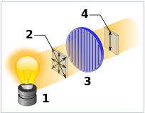
In the above image, the incandescent light bulb $1$ emits completely random polarized photons $2$ with mixed state density matrix.
As mentioned before, an unpolarized light can be explained with an ensemble average i.e. say each photon is either $|R\rangle$ or $|L\rangle$ with $50%$ probability for each. Another possible ensemble average is: each photon is either $\frac{|R\rangle+|L\rangle}{\sqrt 2}$ or $\frac{|R\rangle - |L\rangle}{\sqrt 2}$ with $50\%$ probability for each. There are lots of other possibilities too. Try to come up with some yourself. The point to note is that the density matrix for all these possible ensembles will be exactly the same. And this is exactly the reason why density matrix decomposition into pure states is not unique. Let's check:
Case 1: $50\%$ $|R\rangle$ & $50\%$ $|L\rangle$
$$\rho_{\text{mixed}} = 0.5 |R\rangle \langle R| + 0.5 |L\rangle \langle L|$$
Now, in the basis $\{|R\rangle, |L\rangle\}$, $|R\rangle$ can be denoted as $\begin{bmatrix} 1 \\ 0 \end{bmatrix}$ and $|L\rangle$ can be denoted as $\begin{bmatrix} 0 \\ 1 \end{bmatrix}$
$$\therefore 0.5 \left(\begin{bmatrix} 1 \\ 0 \end{bmatrix} \otimes \begin{bmatrix} 1 & 0 \end{bmatrix}\right) + 0.5 \left(\begin{bmatrix} 0 \\ 1 \end{bmatrix} \otimes \begin{bmatrix} 0 & 1 \end{bmatrix}\right)$$
$$= 0.5 \begin{bmatrix} 1 & 0 \\ 0 & 0 \end{bmatrix} + 0.5\begin{bmatrix} 0 & 0 \\ 0 & 1 \end{bmatrix}$$
$$= \begin{bmatrix} 0.5 & 0 \\ 0 & 0.5 \end{bmatrix}$$
Case 2: $50\%$ $\frac{|R\rangle + |L\rangle}{\sqrt 2}$ & $50\%$ $\frac{|R\rangle - |L\rangle}{\sqrt 2}$
$$\rho_{\text{mixed}} = 0.5 \left(\frac{|R\rangle + |L\rangle}{\sqrt 2}\right)\otimes \left(\frac{\langle R| + \langle L|}{\sqrt 2}\right) + 0.5 \left(\frac{|R\rangle - |L\rangle}{\sqrt 2}\right)\otimes \left(\frac{\langle R| - \langle L|}{\sqrt 2}\right)$$
In the basis $\{\frac{|R\rangle + |L\rangle}{\sqrt 2}, \frac{|R\rangle - |L\rangle}{\sqrt 2}\}$, $\frac{|R\rangle + |L\rangle}{\sqrt 2}$ can be denoted as $\begin{bmatrix} 1 \\ 0 \end{bmatrix}$ and $\frac{|R\rangle - |L\rangle}{\sqrt 2}$ can be denoted as $\begin{bmatrix} 0 \\ 1 \end{bmatrix}$
$$\therefore 0.5 \left(\begin{bmatrix} 1 \\ 0 \end{bmatrix} \otimes \begin{bmatrix} 1 & 0 \end{bmatrix}\right) + 0.5 \left(\begin{bmatrix} 0 \\ 1 \end{bmatrix} \otimes \begin{bmatrix} 0 & 1 \end{bmatrix}\right)$$
$$= 0.5 \begin{bmatrix} 1 & 0 \\ 0 & 0 \end{bmatrix} + 0.5\begin{bmatrix} 0 & 0 \\ 0 & 1 \end{bmatrix}$$
$$= \begin{bmatrix} 0.5 & 0 \\ 0 & 0.5 \end{bmatrix}$$
Thus, we can clearly see that we get the same density matrices in both case 1 and case 2.
However, after passing through the vertical plane polarizer (3), the remaining photons are all vertically polarized (4) and have pure state density matrix:
$$\rho_{\text{pure}} = 1 \left(\frac{|R\rangle + |L\rangle}{\sqrt 2}\right)\otimes \left(\frac{\langle R| + \langle L|}{\sqrt 2}\right) + 0 \left(\frac{|R\rangle - |L\rangle}{\sqrt 2}\right)\otimes \left(\frac{\langle R| - \langle L|}{\sqrt 2}\right) $$
In the basis $\{\frac{|R\rangle + |L\rangle}{\sqrt 2}, \frac{|R\rangle - |L\rangle}{\sqrt 2}\}$, $|R\rangle$ can be denoted as $\begin{bmatrix} 1 \\ 0 \end{bmatrix}$ and $|L\rangle$ can be denoted as $\begin{bmatrix} 0 \\ 1 \end{bmatrix}$
$$\therefore 1 \left(\begin{bmatrix} 1 \\ 0 \end{bmatrix} \otimes \begin{bmatrix} 1 & 0 \end{bmatrix}\right) + 0 \left(\begin{bmatrix} 0 \\ 1 \end{bmatrix} \otimes \begin{bmatrix} 0 & 1 \end{bmatrix}\right)$$
$$= 1 \begin{bmatrix} 1 & 0 \\ 0 & 0 \end{bmatrix} + 0\begin{bmatrix} 0 & 0 \\ 0 & 1 \end{bmatrix}$$
$$= \begin{bmatrix} 1 & 0 \\ 0 & 0 \end{bmatrix}$$
The single qubit case:
If your system contains just a single qubit and you're know that its state $|\psi\rangle = \alpha|0\rangle + \beta|1\rangle$ (where $|\alpha|^2+|\beta|^2$) then you are already sure that the 1-qubit system has the state $|\psi\rangle$ with probability $1$!
In this case, the density matrix will simply be:
$$\rho_{\text{pure}} = 1|\psi\rangle \langle \psi|$$
If you're using the orthonormal basis $\{\alpha|0\rangle + \beta|1\rangle,\beta^*|0\rangle - \alpha^*|1\rangle\}$,
the density matrix will simply be:
$$\begin{bmatrix} 1 & 0 \\ 0 & 0 \end{bmatrix}$$
This is very similar to 'case 2' above, so I didn't show the calculations. You can ask questions in the comments if this portion seems unclear.
However, you could also use the $\{|0\rangle,|1\rangle\}$ basis as @DaftWullie did in their answer.
In the general case for a 1-qubit state, the density matrix, in the $\{|0\rangle,|1\rangle\}$ basis would be:
$$\rho = 1(\alpha |0\rangle + \beta |1\rangle) \otimes (\alpha^* \langle 0| + \beta^* \langle 1|)$$
$$= \begin{bmatrix} \alpha \\ \beta \end{bmatrix} \otimes \begin{bmatrix} \alpha^* & \beta^* \end{bmatrix}$$
$$= \begin{bmatrix} \alpha\alpha^* & \alpha\beta^* \\ \beta\alpha^* & \beta\beta^* \end{bmatrix}$$
Notice that this matrix $\rho$ is idempotent i.e. $\rho = \rho^2$. This is an important property of the density matrices of a pure state and helps us to distinguish them from density matrices of mixed states.
Obligatory exercises:
1. Show that density matrices of pure states can be diagonalized to the form $\text{diag}(1,0,0,...)$.
2. Prove that density matrices of pure states are idempotent.
Sources & References:
[1]: https://en.wikipedia.org/wiki/Density_matrix
[2]: https://physics.stackexchange.com/a/158290
Image Credits:
User Kaidor
on Wikimedia

