Fixed error in the circuit diagram (and the code snippet) itself
Source Link
Niel de Beaudrap
  • 12.4k
  • 1
  • 32
  • 72
  % define initial positions of the quantum wires
  \xdef\dy{1.25}
  \defwire (A) at (0);
  \defwire (B) at ({-\dy});
  \defwire (C) at ({-2*\dy});
  % draw wires
  \xdef\dt{0.8}
  \drawwires [\dt] (15);
  \node  at ($(B-0)!0.5!(B-1)$) {$/$};
  \node  at ($(C-0)!0.5!(C-1)$) {$/$};
  % draw gates
  \gate     (B-2)         [H^{\otimes n}];
  \ctrlgate (B-3) (C-3)   [U];
  \virtgate (A-3);
  \gate     (B-4)         [\mathit{FT}^\dagger];
  \ctrlgate (B-7) (A-7)   [R];
  \virtgate (C-7);
  \gate     (B-10)        [\mathit{FT}];
  \ctrlgate (B-11) (C-11) [U];[U^\dagger];
  \gate     (B-12)        [H^{\otimes n}];
  \virtgate (A-12);
  \meas     (A-14)        [Z];
  % draw input and output labels
  \inputlabel  (A-0)  [\lvert 0 \rangle];
  \inputlabel  (B-0)  [\lvert 0 \rangle^{\otimes n}];
  \inputlabel  (C-0)  [\lvert b \rangle];
  \outputlabel (A-15) [\lvert 1 \rangle];
  \outputlabel (B-15) [\lvert 0 \rangle^{\otimes n}];
  \outputlabel (C-15) [\lvert x \rangle];
Circuit diagramCircuit diagram

  % draw circuit
  \xdef\dt{0.8}
  \drawwires [\dt] (15);
  \node  at ($(B-0)!0.5!(B-1)$) {$/$};
  \node  at ($(C-0)!0.5!(C-1)$) {$/$};
  \gate     (B-2)         [H^{\otimes n}];
  \ctrlgate (B-3) (C-3)   [U];
  \virtgate (A-3);
  \gate     (B-4)         [\mathit{FT}^\dagger];
  \ctrlgate (B-7) (A-7)   [R];
  \virtgate (C-7);
  \gate     (B-10)        [\mathit{FT}];
  \ctrlgate (B-11) (C-11) [U];[U^\dagger];
  \gate     (B-12)        [H^{\otimes n}];
  \virtgate (A-12);
  \meas     (A-14)        [Z];
  % draw input and output labels
  \inputlabel  (A-0)  [\lvert 0 \rangle];
  \inputlabel  (B-0)  [\lvert 0 \rangle^{\otimes n}];
  \inputlabel  (C-0)  [\lvert b \rangle];
  \outputlabel (A-15) [\lvert 1 \rangle];
  \outputlabel (B-15) [\lvert 0 \rangle^{\otimes n}];
  \outputlabel (C-15) [\lvert x \rangle];
  % define initial positions of the quantum wires
  \xdef\dy{1.25}
  \defwire (A) at (0);
  \defwire (B) at ({-\dy});
  \defwire (C) at ({-2*\dy});
  % draw wires
  \xdef\dt{0.8}
  \drawwires [\dt] (15);
  \node  at ($(B-0)!0.5!(B-1)$) {$/$};
  \node  at ($(C-0)!0.5!(C-1)$) {$/$};
  % draw gates
  \gate     (B-2)         [H^{\otimes n}];
  \ctrlgate (B-3) (C-3)   [U];
  \virtgate (A-3);
  \gate     (B-4)         [\mathit{FT}^\dagger];
  \ctrlgate (B-7) (A-7)   [R];
  \virtgate (C-7);
  \gate     (B-10)        [\mathit{FT}];
  \ctrlgate (B-11) (C-11) [U];
  \gate     (B-12)        [H^{\otimes n}];
  \virtgate (A-12);
  \meas     (A-14)        [Z];
  % draw input and output labels
  \inputlabel  (A-0)  [\lvert 0 \rangle];
  \inputlabel  (B-0)  [\lvert 0 \rangle^{\otimes n}];
  \inputlabel  (C-0)  [\lvert b \rangle];
  \outputlabel (A-15) [\lvert 1 \rangle];
  \outputlabel (B-15) [\lvert 0 \rangle^{\otimes n}];
  \outputlabel (C-15) [\lvert x \rangle];

Circuit diagram

  % draw circuit
  \xdef\dt{0.8}
  \drawwires [\dt] (15);
  \node  at ($(B-0)!0.5!(B-1)$) {$/$};
  \node  at ($(C-0)!0.5!(C-1)$) {$/$};
  \gate     (B-2)         [H^{\otimes n}];
  \ctrlgate (B-3) (C-3)   [U];
  \virtgate (A-3);
  \gate     (B-4)         [\mathit{FT}^\dagger];
  \ctrlgate (B-7) (A-7)   [R];
  \virtgate (C-7);
  \gate     (B-10)        [\mathit{FT}];
  \ctrlgate (B-11) (C-11) [U];
  \gate     (B-12)        [H^{\otimes n}];
  \virtgate (A-12);
  \meas     (A-14)        [Z];
  % draw input and output labels
  \inputlabel  (A-0)  [\lvert 0 \rangle];
  \inputlabel  (B-0)  [\lvert 0 \rangle^{\otimes n}];
  \inputlabel  (C-0)  [\lvert b \rangle];
  \outputlabel (A-15) [\lvert 1 \rangle];
  \outputlabel (B-15) [\lvert 0 \rangle^{\otimes n}];
  \outputlabel (C-15) [\lvert x \rangle];
  % define initial positions of the quantum wires
  \xdef\dy{1.25}
  \defwire (A) at (0);
  \defwire (B) at ({-\dy});
  \defwire (C) at ({-2*\dy});
  % draw wires
  \xdef\dt{0.8}
  \drawwires [\dt] (15);
  \node  at ($(B-0)!0.5!(B-1)$) {$/$};
  \node  at ($(C-0)!0.5!(C-1)$) {$/$};
  % draw gates
  \gate     (B-2)         [H^{\otimes n}];
  \ctrlgate (B-3) (C-3)   [U];
  \virtgate (A-3);
  \gate     (B-4)         [\mathit{FT}^\dagger];
  \ctrlgate (B-7) (A-7)   [R];
  \virtgate (C-7);
  \gate     (B-10)        [\mathit{FT}];
  \ctrlgate (B-11) (C-11) [U^\dagger];
  \gate     (B-12)        [H^{\otimes n}];
  \virtgate (A-12);
  \meas     (A-14)        [Z];
  % draw input and output labels
  \inputlabel  (A-0)  [\lvert 0 \rangle];
  \inputlabel  (B-0)  [\lvert 0 \rangle^{\otimes n}];
  \inputlabel  (C-0)  [\lvert b \rangle];
  \outputlabel (A-15) [\lvert 1 \rangle];
  \outputlabel (B-15) [\lvert 0 \rangle^{\otimes n}];
  \outputlabel (C-15) [\lvert x \rangle];

Circuit diagram

  % draw circuit
  \xdef\dt{0.8}
  \drawwires [\dt] (15);
  \node  at ($(B-0)!0.5!(B-1)$) {$/$};
  \node  at ($(C-0)!0.5!(C-1)$) {$/$};
  \gate     (B-2)         [H^{\otimes n}];
  \ctrlgate (B-3) (C-3)   [U];
  \virtgate (A-3);
  \gate     (B-4)         [\mathit{FT}^\dagger];
  \ctrlgate (B-7) (A-7)   [R];
  \virtgate (C-7);
  \gate     (B-10)        [\mathit{FT}];
  \ctrlgate (B-11) (C-11) [U^\dagger];
  \gate     (B-12)        [H^{\otimes n}];
  \virtgate (A-12);
  \meas     (A-14)        [Z];
  % draw input and output labels
  \inputlabel  (A-0)  [\lvert 0 \rangle];
  \inputlabel  (B-0)  [\lvert 0 \rangle^{\otimes n}];
  \inputlabel  (C-0)  [\lvert b \rangle];
  \outputlabel (A-15) [\lvert 1 \rangle];
  \outputlabel (B-15) [\lvert 0 \rangle^{\otimes n}];
  \outputlabel (C-15) [\lvert x \rangle];
Minor revision to make snippet more complete
Source Link
Niel de Beaudrap
  • 12.4k
  • 1
  • 32
  • 72
  % define initial positions of the quantum wires
  \xdef\dy{1.25}
  \defwire (A) at (0);
  \defwire (B) at ({-\dy});
  \defwire (C) at ({-2*\dy});
  % draw wires
  \xdef\dt{0.8}
  \drawwires [\dt] (15);
  \node  at ($(B-0)!0.5!(B-1)$) {$/$};
  \node  at ($(C-0)!0.5!(C-1)$) {$/$};
  % draw gates
  \gate     (B-2)         [H^{\otimes n}];
  \ctrlgate (B-3) (C-3)   [U];
  \virtgate (A-3);
  \gate     (B-4)         [\mathit{FT}^\dagger];
  \ctrlgate (B-7) (A-7)   [R];
  \virtgate (C-7);
  \gate     (B-10)        [\mathit{FT}];
  \ctrlgate (B-11) (C-11) [U];
  \gate     (B-12)        [H^{\otimes n}];
  \virtgate (A-12);
  \meas     (A-14)        [Z];
  % draw input and output labels
  \inputlabel  (A-0)  [\lvert 0 \rangle];
  \inputlabel  (B-0)  [\lvert 0 \rangle^{\otimes n}];
  \inputlabel  (C-0)  [\lvert b \rangle];
  \outputlabel (A-15) [\lvert 1 \rangle];
  \outputlabel (B-15) [\lvert 0 \rangle^{\otimes n}];
  \outputlabel (C-15) [\lvert x \rangle];
  \let\qmwires\empty
  % define initial positions of the quantum wires
  \xdef\dy{1.25}
  \let\qmwires\empty
  \defwire (A) at (0);
  \defwire (B) at ({-\dy});
  \defwire (C) at ({-2*\dy});
  % draw wires
  \xdef\dt{0.8}
  \drawwires [\dt] (15);
  \node  at ($(B-0)!0.5!(B-1)$) {$/$};
  \node  at ($(C-0)!0.5!(C-1)$) {$/$};
  % draw gates
  \gate     (B-2)         [H^{\otimes n}];
  \ctrlgate (B-3) (C-3)   [U];
  \virtgate (A-3);
  \gate     (B-4)         [\mathit{FT}^\dagger];
  \ctrlgate (B-7) (A-7)   [R];
  \virtgate (C-7);
  \gate     (B-10)        [\mathit{FT}];
  \ctrlgate (B-11) (C-11) [U];
  \gate     (B-12)        [H^{\otimes n}];
  \virtgate (A-12);
  \meas     (A-14)        [Z];
  % draw input and output labels
  \inputlabel  (A-0)  [\lvert 0 \rangle];
  \inputlabel  (B-0)  [\lvert 0 \rangle^{\otimes n}];
  \inputlabel  (C-0)  [\lvert b \rangle];
  \outputlabel (A-15) [\lvert 1 \rangle];
  \outputlabel (B-15) [\lvert 0 \rangle^{\otimes n}];
  \outputlabel (C-15) [\lvert x \rangle];
  % define initial positions of the quantum wires
  \xdef\dy{1.25}
  \let\qmwires\empty
  \defwire (A) at (0);
  \defwire (B) at ({-\dy});
  \defwire (C) at ({-2*\dy});
  % define initial positions of the quantum wires
  \xdef\dy{1.25}
  \defwire (A) at (0);
  \defwire (B) at ({-\dy});
  \defwire (C) at ({-2*\dy});
  % draw wires
  \xdef\dt{0.8}
  \drawwires [\dt] (15);
  \node  at ($(B-0)!0.5!(B-1)$) {$/$};
  \node  at ($(C-0)!0.5!(C-1)$) {$/$};
  % draw gates
  \gate     (B-2)         [H^{\otimes n}];
  \ctrlgate (B-3) (C-3)   [U];
  \virtgate (A-3);
  \gate     (B-4)         [\mathit{FT}^\dagger];
  \ctrlgate (B-7) (A-7)   [R];
  \virtgate (C-7);
  \gate     (B-10)        [\mathit{FT}];
  \ctrlgate (B-11) (C-11) [U];
  \gate     (B-12)        [H^{\otimes n}];
  \virtgate (A-12);
  \meas     (A-14)        [Z];
  % draw input and output labels
  \inputlabel  (A-0)  [\lvert 0 \rangle];
  \inputlabel  (B-0)  [\lvert 0 \rangle^{\otimes n}];
  \inputlabel  (C-0)  [\lvert b \rangle];
  \outputlabel (A-15) [\lvert 1 \rangle];
  \outputlabel (B-15) [\lvert 0 \rangle^{\otimes n}];
  \outputlabel (C-15) [\lvert x \rangle];
  \let\qmwires\empty
  % define initial positions of the quantum wires
  \xdef\dy{1.25}
  \defwire (A) at (0);
  \defwire (B) at ({-\dy});
  \defwire (C) at ({-2*\dy});
Added macros to simplify defining the circuit, and to fix non-uniformity of background frame heights
Source Link
Niel de Beaudrap
  • 12.4k
  • 1
  • 32
  • 72

Until such a time as Daftwullie makes his circuit-drawing library public, here is an answer which more-or-less describes the way in which I draw circuits in TiKZ, with some macros to help make the result more reader-friendly.

Edit —

  1. I've revised this answer to make some small improvements in the commands, to tidy up the commands for drawing the wires for instance, because it seemed worthwhile.

  2. Flattering as it is to have this answer be the accepted one for the time being, I think I should point out that the quantikz package (see Daftwullie's answer below) and the qpic package (as pointed out in cnada's answer below) are both libraries with reasonably complete interfaces, and so better for people looking for a quick and simple solution. The code below is probably more suitable for people who are comfortable with TiKZ, and might like to tweak their circuit diagrams with TiKZ commands, but who wouldn't mind having some macros to streamline drawing their diagrams. — Nice as it might be to, for the moment I have no ambition to write a LaTeX package to make these macros available with a nice interface for all purposes (but anyone else who would like to is welcome if they give me some of the credit).

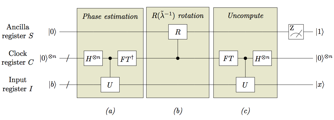
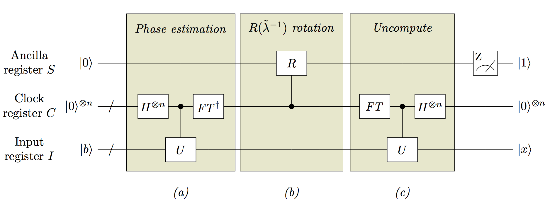
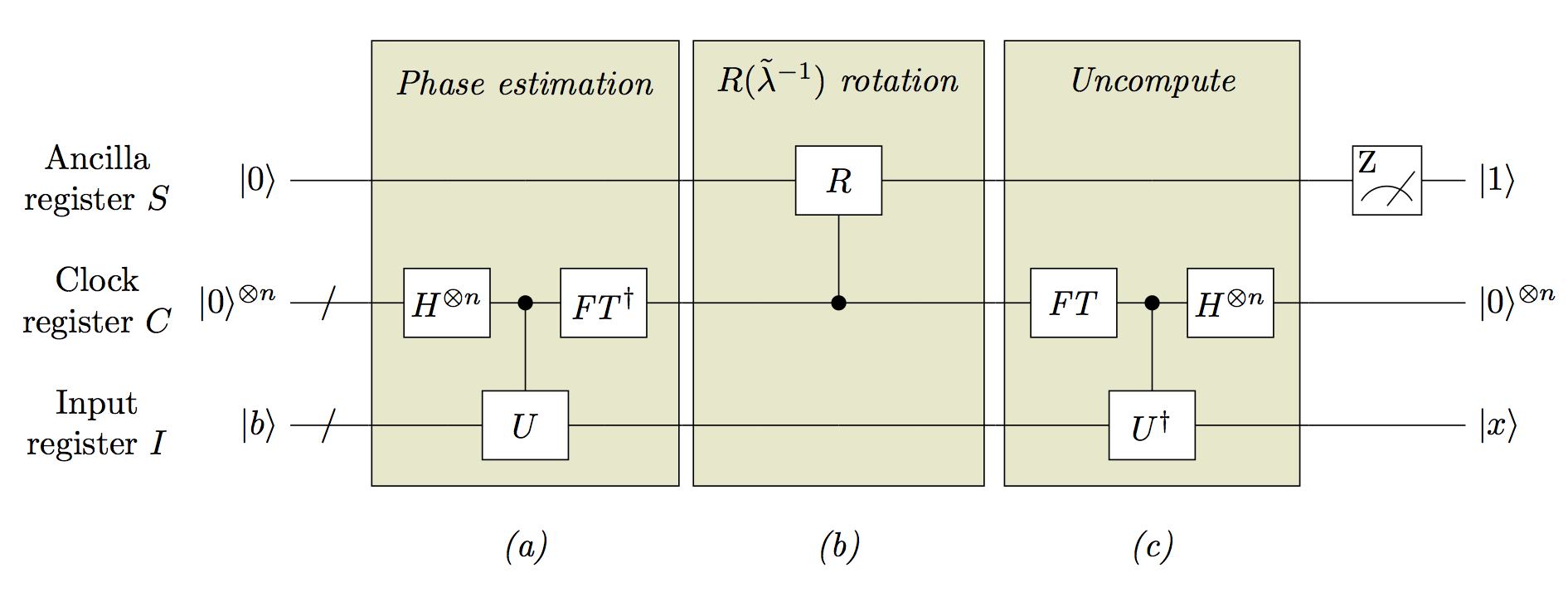
See below for all of the code used to generate this example: the following commands are just the ones used to draw the gates themselves, and the input and output labelscircuit itself. (This snippet involves macros which I have defined for the purpose of this post, which I also define below.)

  % draw circuitwires
  \xdef\dt{0.8}
  \drawwires [\dt] (15);
  \node  at ($(B-0)!0.5!(B-1)$) {$/$};
  \node  at ($(C-0)!0.5!(C-1)$) {$/$};
  % draw gates
  \gate     (B-2)         [H^{\otimes n}];
  \ctrlgate (B-3) (C-3)   [U];
  \virtgate (A-3);
  \gate     (B-4)         [\mathit{FT}^\dagger];
  \ctrlgate (B-7) (A-7)   [R];
  \virtgate (C-7);
  \gate     (B-10)        [\mathit{FT}];
  \ctrlgate (B-11) (C-11) [U];
  \gate     (B-12)        [H^{\otimes n}];
  \virtgate (A-12);
  \meas     (A-14)        [Z];
  % draw input and output labels
  \inputlabel  (A-0)  [\lvert 0 \rangle];
  \inputlabel  (B-0)  [\lvert 0 \rangle^{\otimes n}];
  \inputlabel  (C-0)  [\lvert b \rangle];
  \outputlabel (A-15) [\lvert 1 \rangle];
  \outputlabel (B-15) [\lvert 0 \rangle^{\otimes n}];
  \outputlabel (C-15) [\lvert x \rangle];

Circuit diagramCircuit diagram

\def\inputlabel (#1) [#2]{%
  \node at (#1) [anchor=east] {$#2$}
}
\def\outputlabel (#1) [#2]{%
  \node at (#1) [anchor=west] {$#2$}
}

The macros above are all looking for co-ordinates at which to place the gates. I also define macros to define "wires", which have regularly spaced co-ordinates where gates can be located. The first is a macro which allows you to define a named wire (such as A, B, x3, etc.) and its vertical position in the circuit diagram (these diagrams are left-to-right by default, which you can change most easily using the rotate option of the tikzpicture environment.)

\def\defwire (#1) at (#2){%
  \ifx\qmwires\empty
    \edef\qmwires{#1}%
  \else
    \edef\qmwires{\qmwires,#1}%
  \fi
  \coordinate (#1-0) at ($(0,#2)$)%
}

Having defined a collection of wires, the following command then draws all of them, starting from the same left-most starting point and ending at the same right-most ending point, with increments by a fixed amount (given in the square brackets) and for a given number of time slices. This defines a sequence of 'time-slice' co-ordinates for each wire: for a wire A, it defines the co-ordinates A-0, A-1, and so forth up until A-t (where t is the value of the second argument).

\def\drawwires [#1] (#2);{%
  \xdef\u{0}
  \foreach \t in {0,...,#2} {%
    \foreach \l in \qmwires {%
      \coordinate (\l-\t) at ($(\l-\u) + (#1,0)$);
      \draw (\l-\u) -- (\l-\t);
    }
    \xdef\u{\t}
  }
}
\begin{document}
\begin{tikzpicture}

When you draw a circuit using TiKZ, you will often want to change the spacing a bit. You can do that using macros which are used to define the dimensions of the circuit structure. I arrived at the figures below by trial and error.

  % define diagram parameters
  \xdef\dy{1.25}
  \xdef\dt{0.8}

We now set out some co-ordinates forstart by defining the relative positions of the wires. (For convenience, I am namingdo this using a macro to define the spacing between them, that I can quickly change to adjust the spacing.) Below, I define three wires: A, B, and C, and name some points on the wires after whole-numbered time slices, such as 0, 1, and 2. Thus the first co-ordinates are A-0, B-0, and C-0.

  % define initial positions of the quantum wires
  \coordinate (A-0) at (0,0);
  \coordinate (B-0) at ($(A-0) + (0,-\dy)$);
  \coordinate (C-0) at ($(B-0) + (0,-\dy)$);

I now draw our the wires for the circuit by extending each wire, one time-step at a time, for as many time-steps as I want. Note the use of the macro \t to define the time-slice, and \u as representing the previous time-slice.

  % define coordinates alonginitial eachpositions of the wires for all timesteps
 quantum \xdef\u{0}wires
  \foreach \t in \xdef\dy{0,..1.,1525} {%
    \foreach \l in {A,B,C} {%\let\qmwires\empty
      \coordinate\defwire (\l-\tA) at ($(\l-\u) + (\dt,0)$0);
      \draw\defwire (\l-\uB) --at (\l{-\t\dy});
    }
 \defwire (C) at \xdef\u({\t}
  -2*\dy});

That's the basic structure of the circuit defined. IWe now placedraw the slashes for your two lower registerscircuit, half-way between time-steps 0using the command to draw the wires and 1 (because that's where they lookdefine the best as it turns out)co-ordinates on the wire, and placing gates independently of one another according to those co-ordinates.

  % draw circuit
  \xdef\dt{0.8}
  \drawwires [\dt] (15);
  \node  at ($(B-0)!0.5!(B-1)$) {$/$};
  \node  at ($(C-0)!0.5!(C-1)$) {$/$};

Having done all of this to define the structure of the circuit, I draw the gates, input labels, and output labels for the circuit. Hopefully the commands below are transparent enough.

  % draw circuit
  \gate     (B-2)         [H^{\otimes n}];
  \ctrlgate (B-3) (C-3)   [U];
  \virtgate (A-3);
  \gate     (B-4)         [\mathit{FT}^\dagger];
  \ctrlgate (B-7) (A-7)   [R];
  \virtgate (C-7);
  \gate     (B-10)        [\mathit{FT}];
  \ctrlgate (B-11) (C-11) [U];
  \gate     (B-12)        [H^{\otimes n}];
  \virtgate (A-12);
  \meas     (A-14)        [Z];
  % draw input and output labels
  \inputlabel  (A-0)  [\lvert 0 \rangle];
  \inputlabel  (B-0)  [\lvert 0 \rangle^{\otimes n}];
  \inputlabel  (C-0)  [\lvert b \rangle];
  \outputlabel (A-15) [\lvert 1 \rangle];
  \outputlabel (B-15) [\lvert 0 \rangle^{\otimes n}];
  \outputlabel (C-15) [\lvert x \rangle];
  % draw annotations
  \node [minimum height=4ex] (annotate-1) at ($(A-3) + (0,0.75)$$(A-3) + (0,1)$)
        {\textit{Phase estimation}};
  \node (annotate-a) at ($(C-3) + (0,-1.25)$)
        {\textit{(a)}}; 
 [minimum \nodeheight=4ex] (annotate-2) at ($(A-7) + (0,0.75)$$(A-7) + (0,1)$)
        {\textit{$\smash{R(\tilde\lambda^{-1}})$ rotation}};
  \node [minimum height=4ex] (annotate-3) at ($(A-11) + (0,1)$)
        {\textit{Uncompute}};
  \node (annotate-a) at ($(C-3) + (0,-1.25)$)  {\textit{(a)}}; 
  \node (annotate-b) at ($(C-7) + (0,-1.25)$)
        {\textit{(b)}}; 
  \node (annotate-3) at ($(A-11) + (0,0.75)$)
        {\textit{Uncompute}};
  \node (annotate-c) at ($(C-11) + (0,-1.25)$)
        {\textit{(c)}}; 

Until such a time as Daftwullie makes his circuit-drawing library public, here is an answer which more-or-less describes the way in which I draw circuits in TiKZ, with some macros to help make the result more reader-friendly.

See below for all of the code used to generate this example: the following commands are just the ones used to draw the gates themselves, and the input and output labels. (This snippet involves macros which I have defined for the purpose of this post, which I also define below.)

  % draw circuit
  \gate     (B-2)       [H^{\otimes n}];
  \ctrlgate (B-3) (C-3) [U];
  \virtgate (A-3);
  \gate     (B-4)       [\mathit{FT}^\dagger];
  \ctrlgate (B-7) (A-7) [R];
  \virtgate (C-7);
  \gate     (B-10)       [\mathit{FT}];
  \ctrlgate (B-11) (C-11) [U];
  \gate     (B-12)      [H^{\otimes n}];
  \virtgate (A-12);
  \meas     (A-14)      [Z];
  % draw input and output labels
  \inputlabel  (A-0)  [\lvert 0 \rangle];
  \inputlabel  (B-0)  [\lvert 0 \rangle^{\otimes n}];
  \inputlabel  (C-0)  [\lvert b \rangle];
  \outputlabel (A-15) [\lvert 1 \rangle];
  \outputlabel (B-15) [\lvert 0 \rangle^{\otimes n}];
  \outputlabel (C-15) [\lvert x \rangle];

Circuit diagram

\def\inputlabel (#1) [#2]{%
  \node at (#1) [anchor=east] {$#2$}
}
\def\outputlabel (#1) [#2]{%
  \node at (#1) [anchor=west] {$#2$}
}
\begin{document}
\begin{tikzpicture}

When you draw a circuit using TiKZ, you will often want to change the spacing a bit. You can do that using macros which are used to define the dimensions of the circuit structure. I arrived at the figures below by trial and error.

  % define diagram parameters
  \xdef\dy{1.25}
  \xdef\dt{0.8}

We now set out some co-ordinates for the wires. I am naming the wires A, B, and C, and name some points on the wires after whole-numbered time slices, such as 0, 1, and 2. Thus the first co-ordinates are A-0, B-0, and C-0.

  % define initial positions of the quantum wires
  \coordinate (A-0) at (0,0);
  \coordinate (B-0) at ($(A-0) + (0,-\dy)$);
  \coordinate (C-0) at ($(B-0) + (0,-\dy)$);

I now draw our the wires for the circuit by extending each wire, one time-step at a time, for as many time-steps as I want. Note the use of the macro \t to define the time-slice, and \u as representing the previous time-slice.

  % define coordinates along each of the wires for all timesteps
  \xdef\u{0}
  \foreach \t in {0,...,15} {%
    \foreach \l in {A,B,C} {%
      \coordinate (\l-\t) at ($(\l-\u) + (\dt,0)$);
      \draw (\l-\u) -- (\l-\t);
    }
    \xdef\u{\t}
  }

That's the basic structure of the circuit defined. I now place the slashes for your two lower registers, half-way between time-steps 0 and 1 (because that's where they look the best as it turns out).

  \node  at ($(B-0)!0.5!(B-1)$) {$/$};
  \node  at ($(C-0)!0.5!(C-1)$) {$/$};

Having done all of this to define the structure of the circuit, I draw the gates, input labels, and output labels for the circuit. Hopefully the commands below are transparent enough.

  % draw circuit
  \gate     (B-2)       [H^{\otimes n}];
  \ctrlgate (B-3) (C-3) [U];
  \virtgate (A-3);
  \gate     (B-4)       [\mathit{FT}^\dagger];
  \ctrlgate (B-7) (A-7) [R];
  \virtgate (C-7);
  \gate     (B-10)       [\mathit{FT}];
  \ctrlgate (B-11) (C-11) [U];
  \gate     (B-12)      [H^{\otimes n}];
  \virtgate (A-12);
  \meas     (A-14)      [Z];
  % draw input and output labels
  \inputlabel  (A-0)  [\lvert 0 \rangle];
  \inputlabel  (B-0)  [\lvert 0 \rangle^{\otimes n}];
  \inputlabel  (C-0)  [\lvert b \rangle];
  \outputlabel (A-15) [\lvert 1 \rangle];
  \outputlabel (B-15) [\lvert 0 \rangle^{\otimes n}];
  \outputlabel (C-15) [\lvert x \rangle];
  % draw annotations
  \node (annotate-1) at ($(A-3) + (0,0.75)$)
        {\textit{Phase estimation}};
  \node (annotate-a) at ($(C-3) + (0,-1.25)$)
        {\textit{(a)}}; 
  \node (annotate-2) at ($(A-7) + (0,0.75)$)
        {\textit{$\smash{R(\tilde\lambda^{-1}})$ rotation}};
  \node (annotate-b) at ($(C-7) + (0,-1.25)$)
        {\textit{(b)}}; 
  \node (annotate-3) at ($(A-11) + (0,0.75)$)
        {\textit{Uncompute}};
  \node (annotate-c) at ($(C-11) + (0,-1.25)$)
        {\textit{(c)}}; 

Edit —

  1. I've revised this answer to make some small improvements in the commands, to tidy up the commands for drawing the wires for instance, because it seemed worthwhile.

  2. Flattering as it is to have this answer be the accepted one for the time being, I think I should point out that the quantikz package (see Daftwullie's answer below) and the qpic package (as pointed out in cnada's answer below) are both libraries with reasonably complete interfaces, and so better for people looking for a quick and simple solution. The code below is probably more suitable for people who are comfortable with TiKZ, and might like to tweak their circuit diagrams with TiKZ commands, but who wouldn't mind having some macros to streamline drawing their diagrams. — Nice as it might be to, for the moment I have no ambition to write a LaTeX package to make these macros available with a nice interface for all purposes (but anyone else who would like to is welcome if they give me some of the credit).

See below for all of the code used to generate this example: the following commands are just the ones used to draw the circuit itself. (This snippet involves macros which I have defined for the purpose of this post, which I also define below.)

  % draw wires
  \xdef\dt{0.8}
  \drawwires [\dt] (15);
  \node  at ($(B-0)!0.5!(B-1)$) {$/$};
  \node  at ($(C-0)!0.5!(C-1)$) {$/$};
  % draw gates
  \gate     (B-2)         [H^{\otimes n}];
  \ctrlgate (B-3) (C-3)   [U];
  \virtgate (A-3);
  \gate     (B-4)         [\mathit{FT}^\dagger];
  \ctrlgate (B-7) (A-7)   [R];
  \virtgate (C-7);
  \gate     (B-10)        [\mathit{FT}];
  \ctrlgate (B-11) (C-11) [U];
  \gate     (B-12)        [H^{\otimes n}];
  \virtgate (A-12);
  \meas     (A-14)        [Z];
  % draw input and output labels
  \inputlabel  (A-0)  [\lvert 0 \rangle];
  \inputlabel  (B-0)  [\lvert 0 \rangle^{\otimes n}];
  \inputlabel  (C-0)  [\lvert b \rangle];
  \outputlabel (A-15) [\lvert 1 \rangle];
  \outputlabel (B-15) [\lvert 0 \rangle^{\otimes n}];
  \outputlabel (C-15) [\lvert x \rangle];

Circuit diagram

\def\inputlabel (#1) [#2]{%
  \node at (#1) [anchor=east] {$#2$}
}
\def\outputlabel (#1) [#2]{%
  \node at (#1) [anchor=west] {$#2$}
}

The macros above are all looking for co-ordinates at which to place the gates. I also define macros to define "wires", which have regularly spaced co-ordinates where gates can be located. The first is a macro which allows you to define a named wire (such as A, B, x3, etc.) and its vertical position in the circuit diagram (these diagrams are left-to-right by default, which you can change most easily using the rotate option of the tikzpicture environment.)

\def\defwire (#1) at (#2){%
  \ifx\qmwires\empty
    \edef\qmwires{#1}%
  \else
    \edef\qmwires{\qmwires,#1}%
  \fi
  \coordinate (#1-0) at ($(0,#2)$)%
}

Having defined a collection of wires, the following command then draws all of them, starting from the same left-most starting point and ending at the same right-most ending point, with increments by a fixed amount (given in the square brackets) and for a given number of time slices. This defines a sequence of 'time-slice' co-ordinates for each wire: for a wire A, it defines the co-ordinates A-0, A-1, and so forth up until A-t (where t is the value of the second argument).

\def\drawwires [#1] (#2);{%
  \xdef\u{0}
  \foreach \t in {0,...,#2} {%
    \foreach \l in \qmwires {%
      \coordinate (\l-\t) at ($(\l-\u) + (#1,0)$);
      \draw (\l-\u) -- (\l-\t);
    }
    \xdef\u{\t}
  }
}
\begin{document}
\begin{tikzpicture}

We start by defining the relative positions of the wires. (For convenience, I do this using a macro to define the spacing between them, that I can quickly change to adjust the spacing.) Below, I define three wires: A, B, and C.

  % define initial positions of the quantum wires
  \xdef\dy{1.25}
  \let\qmwires\empty
  \defwire (A) at (0);
  \defwire (B) at ({-\dy});
  \defwire (C) at ({-2*\dy});

We now draw the circuit, using the command to draw the wires and define the co-ordinates on the wire, and placing gates independently of one another according to those co-ordinates.

  % draw circuit
  \xdef\dt{0.8}
  \drawwires [\dt] (15);
  \node  at ($(B-0)!0.5!(B-1)$) {$/$};
  \node  at ($(C-0)!0.5!(C-1)$) {$/$};
  \gate     (B-2)         [H^{\otimes n}];
  \ctrlgate (B-3) (C-3)   [U];
  \virtgate (A-3);
  \gate     (B-4)         [\mathit{FT}^\dagger];
  \ctrlgate (B-7) (A-7)   [R];
  \virtgate (C-7);
  \gate     (B-10)        [\mathit{FT}];
  \ctrlgate (B-11) (C-11) [U];
  \gate     (B-12)        [H^{\otimes n}];
  \virtgate (A-12);
  \meas     (A-14)        [Z];
  % draw input and output labels
  \inputlabel  (A-0)  [\lvert 0 \rangle];
  \inputlabel  (B-0)  [\lvert 0 \rangle^{\otimes n}];
  \inputlabel  (C-0)  [\lvert b \rangle];
  \outputlabel (A-15) [\lvert 1 \rangle];
  \outputlabel (B-15) [\lvert 0 \rangle^{\otimes n}];
  \outputlabel (C-15) [\lvert x \rangle];
  % draw annotations
  \node [minimum height=4ex] (annotate-1) at ($(A-3) + (0,1)$)
        {\textit{Phase estimation}};
  \node [minimum height=4ex] (annotate-2) at ($(A-7) + (0,1)$)
        {\textit{$\smash{R(\tilde\lambda^{-1}})$ rotation}};
  \node [minimum height=4ex] (annotate-3) at ($(A-11) + (0,1)$)
        {\textit{Uncompute}};
  \node (annotate-a) at ($(C-3) + (0,-1.25)$)  {\textit{(a)}}; 
  \node (annotate-b) at ($(C-7) + (0,-1.25)$)  {\textit{(b)}}; 
  \node (annotate-c) at ($(C-11) + (0,-1.25)$) {\textit{(c)}};
Corrected typo in choice of ams library
Source Link
Niel de Beaudrap
  • 12.4k
  • 1
  • 32
  • 72
Loading
Source Link
Niel de Beaudrap
  • 12.4k
  • 1
  • 32
  • 72
Loading